In the following chapter we want to give some examples on how to model a machine vision system using definitions from Part2.
As base for the examples, we use the vision system setup shown below.
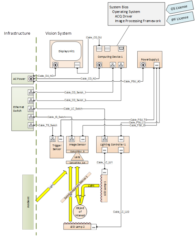
Figure 49 – An example Machine Vision System
Within a machine, its components are usually mounted / mechanically connected in some way. Part2 allows you to express the information, how and where things are mounted.
Let us model a simple example:
A camera is usually built out of a camera body (which we will represent by the image sensor as its most important functional part) and a lens that creates a projection on that sensor.
Using the object types given above, we would get an image sensor object and a lens object located in their specific folders.
As the lens is attached to the outside of the camera body, and in principle can be detached, we will use the HasAttachedComponent Reference to show this relationship between the two objects
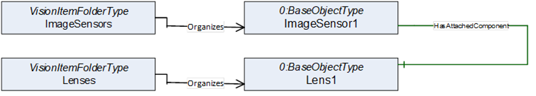
Figure 50 – Mechanical Connections with OPC UA References
Browsing this model, we get the information that a lens called “Lens1” is attached to an image sensor called “ImageSensor1”.
Now let us mount an optical filter onto the lens. This can be done using the same modeling approach.
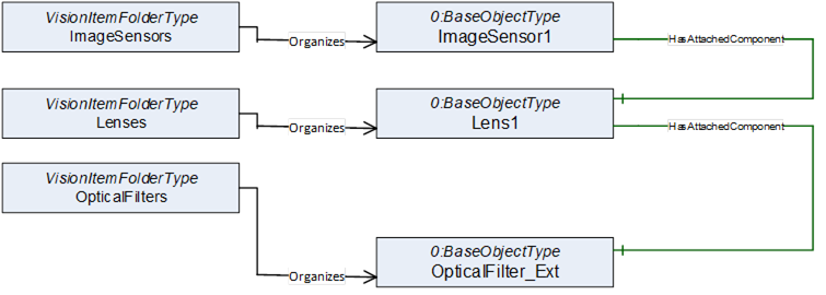
Figure 51 – Mechanical Connections with OPC UA References
Let us assume the image sensor is equipped with an internal infrared filter in front of the actual sensor chip. As this filter is an integral part of the image sensor, there is no need to add it to the model at all, as the image sensor is already in the model.
But maybe we want to make sure that a service guy browsing this model during maintenance work is aware of the presence of that IR filter. Therefore, we can add it to the model, this time using the HasContianedComponent reference expressing that something is an integral, i.e., not easily removable, part of some other component.
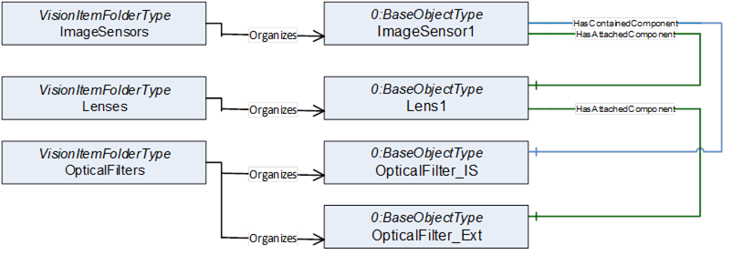
Figure 52 – Mechanical Connections with OPC UA References
Maybe if someone later on will have to replace the lens it would be nice to know which mechanical interface (like C-Mount or F-Mount) is used in this assembly.
Part2 allows you to get into more detail by adding additional information layers to the model. To add information about the physical connection types supported by your components you may add objects naming each of this physical interfaces / connection points located at your item.
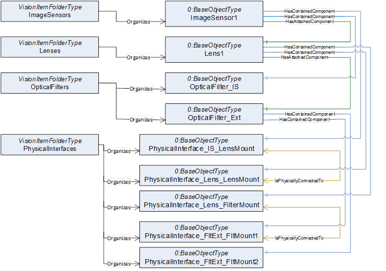
Figure 53 – Mechanical Connections with OPC UA References
Browsing this model we get the information that there is a lens mount built into the Image sensor. The PhysicalInterface_IS_LensMount Object can hold all information you may need to specify what type of mount this is.
Further browsing shows that Lens1 has two physical connection ports. There is a lens mount on one end and a filter mount on the other.
We also see that the Filter has two filter mounts (on both sides) to be able to stack multiple filters if needed.
During engineering of the system, you may compare the image sensor1 lens mount to the lens1 lens mount to see if the components will fit together.
As this example shows an already mounted lens - as we can see by the HasAttachedComponent reference between image sensor and lens - we will find this information reflected also by the additional information layer of the physical ports. This time we find an IsPhysicallyConnectedTo reference between the two lens mount objects.
The nature of physical ports is that they may be connected or disconnected several times. Therefore, at this level we are only using the IsPhysicallyConnectedTo reference which expresses a somehow weak relation – it is currently physically connected, but this could change at any time. Despite of that, at the component level above you still have the much stronger HasAttachedComponent reference which tells you that this is a connection not intended to be broken during normal operation.
Part 2 offers an additional method of giving your service department information about what they should or should not try to disassemble on site during maintenance. It introduces the possibility to add a service class tag to the components, which gives information about what parts of the machine may be disassembled at the customer site and which components should only be removed as an assembly where you do not disassemble individual components.
So, let’s say you know that the system will be working in a dusty environment, possibly with oil mist in the air. Therefore, it is probably not a good idea to remove the lens from the image sensor at the production site as there is a high risk to render the image sensor useless because oil is deposited on it.
The service class standard originating from aircraft maintenance, but now used in a wide field of applications, defines some standard labels like “line replaceable unit” – this component may be removed at the customer site – and “shop replaceable unit” – this component should not be removed at a customer site; only at your workshop you are supposed to dismantle this assembly.
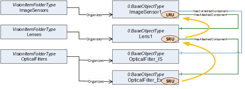
Figure 54 – Service Class Tags
By tagging the components you can give your service guys some information how to handle a repair. If the filter mounted on the lens gets damaged, you can browse the following information from the model:
the filter is tagged SRU – do not remove
the filter is attached to the lens, the lens is tagged SRU – do not remove
the lens is attached to the image sensor, that is tagged LRU – remove this assembly
Therefore, the service technician should remove the sensor together with the lens and filter mounted to it and take it back to the repair shop to replace the damaged filter.
Some devices / components itself are built in a modular way. For example, an IPC usually is shown as a unit within the system, but internally it uses standardized modules like a PCIe plug-in card or a 2,5” solid state drive. It may be worthwhile to be able to name these modules for maintenance purposes.
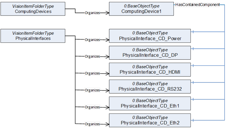
Figure 55 – Modular Devices with OPC UA References
In the example above, we see an industrial computer together with its connectors that are named such that it is possible to show the connectivity within the MV system later on.
In this example, the IPC offers connectors for power supply, video output (Display Port and HDMI), a serial interface and two Ethernet Ports.
Most of these interfaces are built into the IPC (soldered to the mainboard). Therefore, we see HasContainedComponent references pointing from the ComputingDevice to the PhysicalInterface nodes which expresses a “this is an integral part of something” relation.
As in the Image sensor example above, it is up to you to decide what internal components are useful to be included in the model. If an internal component has meaningful maintenance information that may be monitored without the context of the device it belongs to, it may be worth it to add that component to the system model.
An example for that could be a hard disk or solid-state drive which usually provides health information (SMART / GPL) often including a prediction if this drive will fail in the near future.
You may incorporate this SMART data into the health information of the device containing the drive, but for a client it could be easier to have a standardized browse point (folder) where to find all SMART data from all drives no matter in which component they are located.
(Note: Part2 does not include a definition for mass storage devices as there are already standards for that)
Another example could be cooling fans. Instead of distributing their maintenance information over the components they are mounted to, it could make monitoring easier to have them all in one folder.
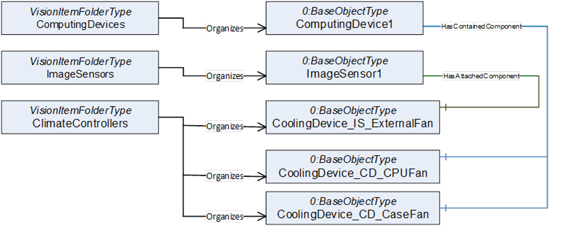
Figure 56 – Modular Devices with OPC UA References
Again, choosing different reference types can be used to give more information on the service task that has to be expected if a part needs to be replaced.
In this example, the Image sensor has an externally attached fan which, by definition of that reference type, should not be hard to detach.
The IPC has a built in CPU fan, which by definition of that reference type Is not designed for easy replacement and it has a contained case fan which is in between those, maybe like a fan cassette of a rack device that may easily be replaced from the outside without the need to dismantle the IPC.
The OPC base specification offers several reference types to describe the relation between software and hardware components.
Below is an example of an IPC running some image processing software framework. To build the model, the first thing is to decide which software components should be named in the model. We here tried to include the things needed for an application that could be updated independently. Therefore, it makes sense to give some version information for those components to be able to keep track of their compatibility if they are updated during normal maintenance operations.
- The Firmware / BIOS of the IPC is needed to run the computer, of course it must fit to the hardware of the IPC.
- The operating system is usually provided as a software image (e.g., backup of the system drive). To be able to run on the IPC it often needs specific BIOS settings and functionality.
- Usually, you need some driver software to adapt the OS to the hardware of the computer and its periphery
- Installed to the OS you will have some application software packages, like the Image processing framework or some service tools. These programs may be started or stopped during normal operation
- To legally use some of the software components like the OS or the Image processing software you usually need software licenses that may have a digital and/or physical representation (license dongle)
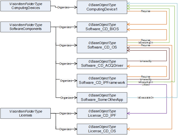
Figure 57 – Software and Licenses
We now will have to add information about the relationships of the named components.
This can be difficult, as it is often hard to decide if a software is “running on” or “hosted by” something or if it “requires” or “utilizes” another component.
There is no right or wrong here, it mainly depends on what aspect you need to make visible to fulfill your monitoring and maintenance needs. And if you can’t decide it is always possible to show multiple aspects by using different reference types in parallel.
The model does not necessarily have to be complete; it is often more helpful to limit it to the important information / relations.
To give you an impression, here are some thoughts why we did put the example together in this specific way:
- If a BIOS update is to be done, we need to check compatibility. The BIOS has to fit to the hardware, but also its configuration has to fit to the OS image running on that machine. Therefore, we decided to show the aspect that the hardware as well as the OS has requirements on the BIOS distributed. The knowledge that a firmware runs on the hardware it is installed on is somehow trivial and therefore we decided to skip that relation.
- If you want to keep track of different versions of the OS Images you did distribute to your system over time, there may be more than one OS Image entity present in the software folder. Therefore, we decided to use the “is executing on” reference to show that the OS image shown in the model is currently running on the IPC.
- A driver package distributed often includes drivers for multiple versions of operating systems (e.g. Windows 10 and 11). Therefore, we did use an “IsHostedBy” to express that in this application the driver package runs on a specific OS Version.
- The Image processing framework may be connected only loosely to the specific IPC and OS Image but instead run on “one available machine” (virtual environments, Docker etc.). Therefore, we used the “IsHostedBy” reference to connect it to the OS and the “IsExecutingOn” reference to show where it is currently executed. This may change during runtime if it becomes assigned to a different IPC.
- The “OtherApp” is currently not executed, but if needed it could run on the IPC, which is indicated by the “IsExecutableOn” reference.
- The OS may need a unique license key, which makes a one-to-one relation between the OS and the license. This is shown by the “Requires” reference. This OS needs this specific key.
- The Image processing Framework may use some kind of “floating license” model. A license dongle allows to run up to a specific number of Image processing Frameworks in parallel no matter on which IPC they are executed. Therefore, we here used the “Utilizes” reference to express that, as long as it is executed, the framework uses up one of these floating licenses.
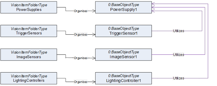
The Utilizes reference is often used in conjunction with shared resources.
In the example below we have a power supply unit with a single power output.
Three devices are connected to that output and therefore share that resource.
This is modeled by Utilizes references.
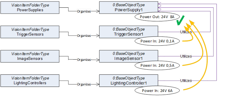
The references now can be used to aggregate information for resource planning.
If you have to select a replacement PSU during repair, you can follow the Utilizes references pointing to the power output in reverse to find the power needs of the three devices and aggregate them to get the requirements for the power supply.
But not in all cases resources are directly used, there could be hidden indirect relations.
A lighting controller often controls an LED lamp by modulating the electrical current to the lamp.
Although there is no direct cable connection between lamp and PSU the lamp is indirectly supplied by the PSU. Normally the power need of the lamp therefore is incorporated into the power need of the lighting controller.
If it is instead needed to explicitly model the relation between lamp and PSU this can be done by adding an additional Utilizes reference (dotted line).
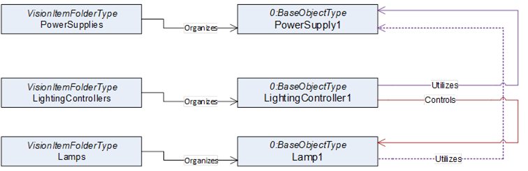
Please be aware that an OPC UA reference cannot have additional parameters. It is simply there or is not there. Therefore, by browsing the references a client cannot distinguish between a reference modeling a direct or indirect relationship (solid line vs. dotted line).
If this is needed a reference refinement must be used to further describe the nature of the dotted Utilizes reference.
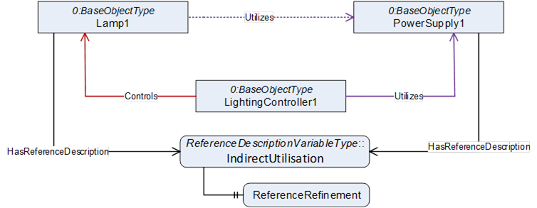
Figure 61 – Reference Refinement of the Utilizes Reference
ReferenceDescription Value of IndirectUtilisation
SourceNode:Lamp1
ReferenceType:Utilizes
IsForward: TRUE
TargetNode:PowerSupply1
ReferenceRefinement of IndirectUtilisation
{
ReferenceListEntry
ReferenceType:Controls
IsForward: FALSE
TargetNode:LightingController1;
ReferenceListEntry
ReferenceType:Utilizes
IsForward: TRUE
TargetNode:PowerSupply1;
};
The refinement allows to give an ordered list of references (a path) that are simplified by the reference the refinement belongs to.
The dotted Utilizes reference is a simpler model of the real path that leads from the lamp to the power supply. In reality, Lamp1 receives its power from the lighting controller (which is expressed by the Controls reference from lighting controller to lamp) and the lighting controller gets its power from the power supply.
Typically, in real world applications a connector of one device is not plugged directly into the connector of another device. You will find a piece of cable in between.
As cables are often a delicate part of a system and could be worn down if connected to a moving machine part, it can be helpful to get information what kind of cable is used and where it is connected directly from the system. Be aware that a cable can have more than two ends (Y-Cable, Bus Cable, Cable Tree).
Part2 allows you to include information in the model as needed, from basic items to in depth detail.
In the example above we saw a Controls reference between the lighting controller and Lamp1.
Now we will add a cable to the model that provides this control connection.
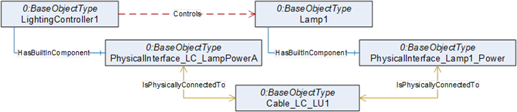
As in the last example we now have two paths from Controller to lamp that stand for the same relation. We again may use a reference refinement to give the information that the Controls reference is provided by that cable connection.
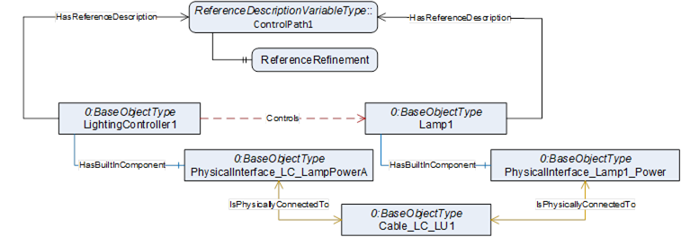
Figure 63 – Reference Refinement of the Controls Reference
ReferenceDescription Value of ControlPath1
SourceNode:LightingController1
ReferenceType:Controls
IsForward: TRUE
TargetNode:Lamp1
ReferenceRefinement of ControlPath1
{
ReferenceListEntry
ReferenceType:HasContianedComponent
IsForward: TRUE
TargetNode:PhysicalInterface_ LC_LampPowerA
ReferenceListEntry
ReferenceType:IsPhysicallyConnectedTo
IsForward: TRUE
TargetNode:Cable_LC_LU1;
ReferenceListEntry
ReferenceType:IsPhysicallyConnectedTo
IsForward: TRUE
TargetNode:PhysicalInterface_Lamp1_Power;
ReferenceListEntry
ReferenceType:HasContianedComponent
IsForward: FALSE
TargetNode:Lamp1;
};
Such control flows often include multiple devices which are part of the communication. If the IPC sends a software trigger to the lighting controller via an Ethernet connection, the signal may have to pass an Ethernet switch. Modeling such details gives you the possibility to do sophisticated error analysis later.
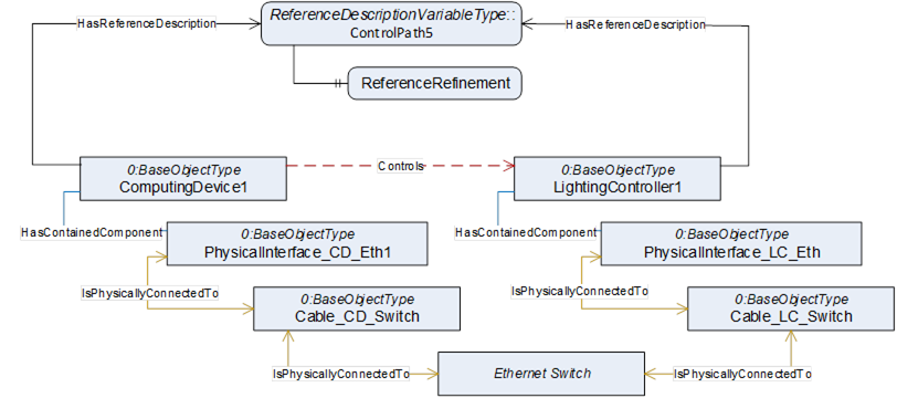
Figure 64 – Reference Refinement of the Controls Reference
ReferenceDescription Value of ControlPath5
SourceNode:ComputingDevice1
ReferenceType:Controls
IsForward: TRUE
TargetNode:LightingController1
ReferenceRefinement of ControlPath5
{
ReferenceListEntry
ReferenceType:HasContianedComponent
IsForward: TRUE
TargetNode:PhysicalInterface_CD_Eth;
ReferenceListEntry
ReferenceType:IsPhysicallyConnectedTo
IsForward: TRUE
TargetNode:Cable_CD_Switch;
ReferenceListEntry
ReferenceType:IsPhysicallyConnectedTo
IsForward: TRUE
TargetNode:Ethernet Switch;
ReferenceListEntry
ReferenceType:IsPhysicallyConnectedTo
IsForward: TRUE
TargetNode:Cable_LC_Switch;
ReferenceListEntry
ReferenceType:IsPhysicallyConnectedTo
IsForward: TRUE
TargetNode:PhysicalInterface_LC_Eth;
ReferenceListEntry
ReferenceType:HasContianedComponent
IsForward: FALSE
TargetNode:LightingController1;
};
If the IPC is currently unable to control the lighting controller, the reference refinement provides the information that a service technician not only will have to check the IPC and the controller, but that there are two cables and an Ethernet switch involved that could be causing the problem.
Using the same modeling approach as described above you can easily add an additional information layer giving detailed information on the connectors and pinout of the cables in the system. If needed, you may even provide a full cabling plan for the whole system.
The models are simple but will become very large (you often hear people saying otherwise, but no, size and complexity are not the same thing).
Please keep in mind that such models are not intended to be made or read by human beings. A cabling plan will be an output of your engineering software and should be read by a service tool helping a service technician doing maintenance or error analysis.
The first thing to do is to add some connectors to the cable model.
Below is an example of a Y-cable with one connector on one end that is split to 2 connectors on the other end.
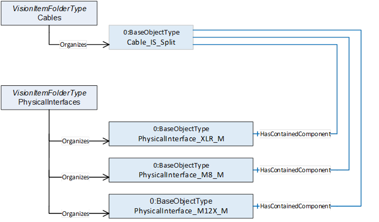
Figure 65 – Detailed modelling of cables
To show the pinout of the connectors we add the wires of the cable to the Cables folder and the pins of the connectors to the PhysicalInterfaces folder. We use the IsPhysicallyConnectedTo reference type to show how everything is wired.
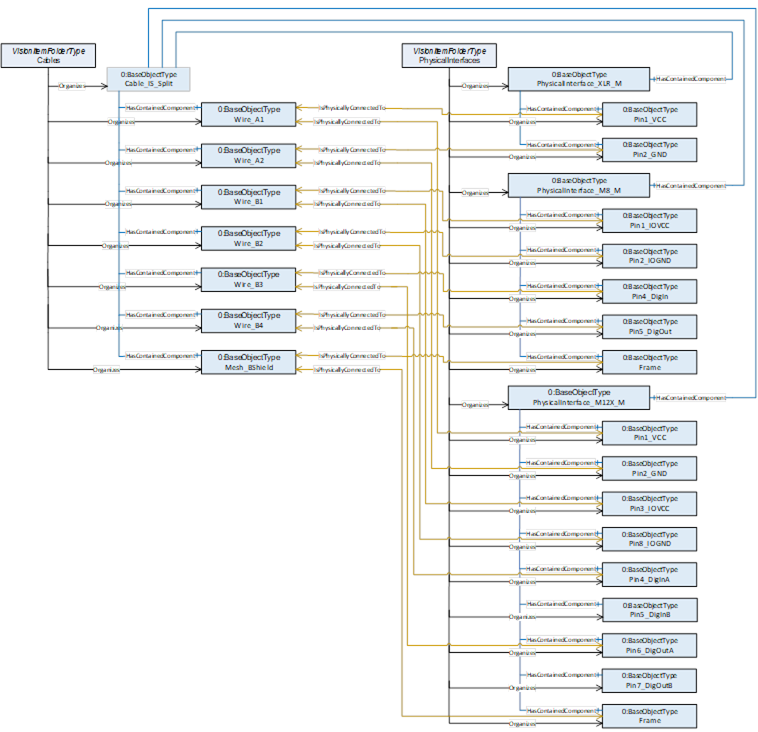
Figure 66 – Detailed modelling of cables
If the cable gets connected to a device, you may decide at which level of information depth you reflect this. The connector of the cable gets physically connected to the fitting connector of the device. You may also show that each pin gets connected which may make it easier to browse large cable trees later on.
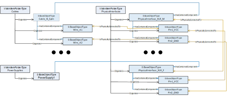
Figure 67 – Detailed modelling of cables
Note: In industrial applications it is common to use screw terminals instead of connectors to connect cables. But even in this case you often need to give detail information on how this end of the cable has to be manufactured. Do you simply have to strip the isolation, or do you need to put on a cable shoe and if yes what type and size of shoe is needed?
An “Open End” object (analog to a pin object) would be a good place to store such information.
In the good ol’ days of image processing it was common practice to use specialized interface cards (framegrabbers) to connect an image sensor to a computing unit. But as the consumer grade interfaces included in nearly all computers kept evolving over time they today are often “good enough” and much cheaper than specialized hardware you have to add to the IPC.
So we now mostly use Ethernet or even USB ports to do image acquisition.
Whereas a frame grabber usually comes with detailed information on which image format and acquisition bandwidth it can handle, you rarely will find such information on a generic USB or Ethernet port. We could have added this kind of data elements to a machine vision specific definition of such ports to close that gap, but we did not find this very useful.
Such generic port types are widely used and there will be definitions how to describe them outside of the image processing world.
Instead, we decided to keep the information that is specific to image processing applications in a separate object that may be attached to a port using a reference.
Even in such a scenario you may want to have a frame grabber entity, even if this is now a software instead of a hardware component, whose hardware aspects are hosted by another physical interface.
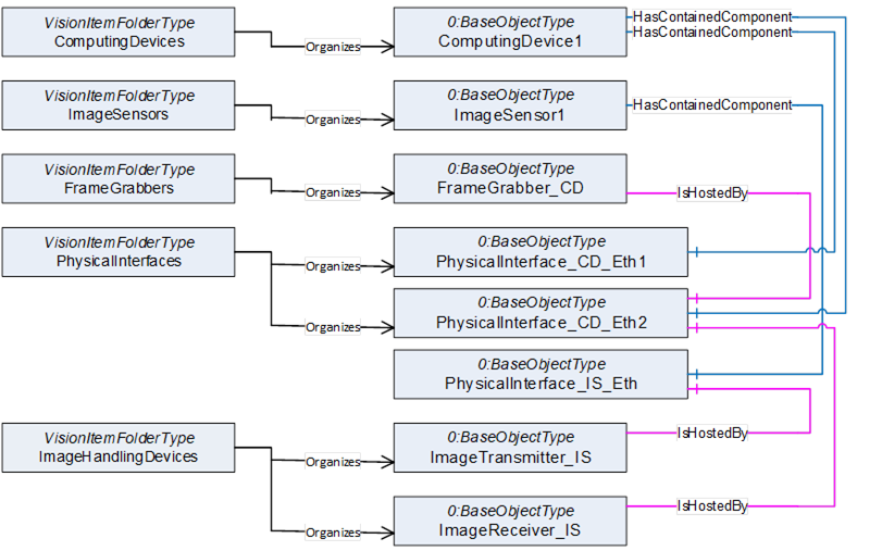
Figure 68 – Image Transceivers
This approach has a big advantage. As consumer interfaces are usually very cheap, modern IPCs come with a lot of them. Often it does not really matter which Ethernet or which USB port the camera is connected to as they are technically identical. So you have some built in redundancy. If you decide to connect the image sensor to Ethernet Port1 instead of Port2, no objects in the model need to be changed. Simply the two “IsHostedBy” references need to be shifted to the other Ethernet port.
As we saw above, our models show relations between devices / components. We may add further layers of information to give more details, e.g., to show that a control flow between devices is dependent on cables connecting them.
In a machine vision system, we do not only care about electrical signals being distributed.
We also care about the distribution of light to be able to answer questions like:
Why do I get no image?
Why is the image I get not as bright as expected?
To be able to model optical relations we introduced an additional reference type called OpticalPath for that purpose.
Note: As our Industry is called machine vision, we use to speak of images coming from a sensor. This could be something like a photo, but often it is something different which would not be called an image in everyday circumstances.
In the same way we use the terms light and optics in a very general way. “Light” can be anything you use to get your “image”, it could be Infrared light, could be X-ray or could even be a sound wave. Everything used to guide or manipulate your “source signal” we call “optical equipment” and the source of that signal we call “lamp”.
We also introduced an SurroundingEnvironment Object. In real world applications you often struggle with the surrounding environment around your Vision System. Maybe you make use of ambient light to make your images or maybe scattered ambient light ruins your image processing if you can’t isolate the system well enough.
In both cases, it is very often necessary to monitor “surrounding environment quality”, meaning the influence the surroundings have on your application (e.g., brightness of ambient light, ambient temperature).
The surrounding environment object is the right place to store such information.
A similar object is the AcquisitionBackground. If for example you need to be able to correctly “see” the contour of an object of interest, you will have some requirements on what is behind that object. So often the background is monitored to warn about dirt and debris showing up before it influences the quality of your image processing. As the acquisition background is often a part of the system (e.g., a gray sheet of metal or a backlight) we distinguished it from the surrounding environment, that is what we find around the vision system.
But back to the optical path.
In the example vision system shown at the beginning of this chapter we can identify 3 main optical paths via which light can reach the image sensor.
- Lamp1 in conjunction with a semitransparent mirror is used to illuminate the surface of our object of interest.
- A backlight Lamp2 is used to be able to see the contour of the object. Some of that light is lost as it has to pass the mirror used for front face illumination
- Stray light from the surrounding environment may disturb our image, as it is not completely blocked in that application
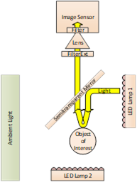
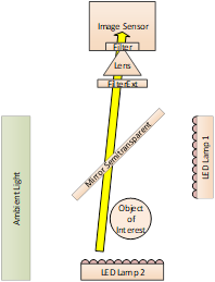
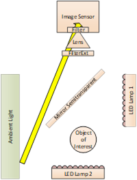
Figure 69 – Optical Paths in the example
This gives us the following model
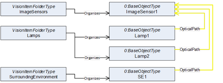
Figure 70 – Modelling of Optical Paths
Using the same approach as we did with the cables we now can include all intermediate objects that are part of these paths of light. As shown above to express a “Path” we need to use reference refinements to give the single references an order to build a path.
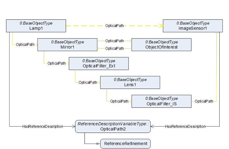
Figure 71 – Optical Path 1: Lamp 1 to Image Sensor
ReferenceDescription Value of OpticalPath1
SourceNode:Lamp1
ReferenceType:OpticalPath
IsForward:TRUE
TargetNode:ImageSensor1
ReferenceRefinement of OpticalPath3
{
ReferenceListEntry
ReferenceType:OpticalPath
IsForward:TRUE
TargetNode:Mirror1;
ReferenceListEntry
ReferenceType:OpticalPath
IsForward:TRUE
TargetNode:ObjectOfInterest;
ReferenceListEntry
ReferenceType:OpticalPath
IsForward:TRUE
TargetNode:Mirror1;
ReferenceListEntry
ReferenceType:OpticalPath
IsForward:TRUE
TargetNode:OpticalFilter_Ext;
ReferenceListEntry
ReferenceType:OpticalPath
IsForward:TRUE
TargetNode:Lens1;
ReferenceListEntry
ReferenceType:OpticalPath
IsForward:TRUE
TargetNode:OpticalFilter_IS;
ReferenceListEntry
ReferenceType:OpticalPath
IsForward:TRUE
TargetNode:ImageSensor1;
};
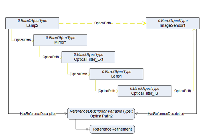
Figure 72 – Optical Path 2: Lamp 2 to Image Sensor
ReferenceDescription Value of OpticalPath2
SourceNode:Lamp2
ReferenceType:OpticalPath
IsForward:TRUE
TargetNode:ImageSensor1
ReferenceRefinement of OpticalPath2
{
ReferenceListEntry
ReferenceType:OpticalPath
IsForward:TRUE
TargetNode:Mirror1;
ReferenceListEntry
ReferenceType:OpticalPath
IsForward:TRUE
TargetNode:OpticalFilter_Ext;
ReferenceListEntry
ReferenceType:OpticalPath
IsForward:TRUE
TargetNode:Lens1;
ReferenceListEntry
ReferenceType:OpticalPath
IsForward:TRUE
TargetNode:OpticalFilter_IS;
ReferenceListEntry
ReferenceType:OpticalPath
IsForward:TRUE
TargetNode:ImageSensor1;
};
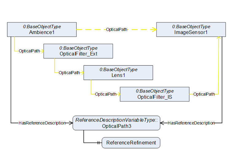
Figure 73 – Optical Path 3: Ambience to Image Sensor
ReferenceDescription Value of OpticalPath3
SourceNode:Ambience1
ReferenceType:OpticalPath
IsForward:TRUE
TargetNode:ImageSensor1
ReferenceRefinement of OpticalPath3
{
ReferenceListEntry
ReferenceType:OpticalPath
IsForward:TRUE
TargetNode:OpticalFilter_Ext;
ReferenceListEntry
ReferenceType:OpticalPath
IsForward:TRUE
TargetNode:Lens1;
ReferenceListEntry
ReferenceType:OpticalPath
IsForward:TRUE
TargetNode:OpticalFilter_IS;
ReferenceListEntry
ReferenceType:OpticalPath
IsForward:TRUE
TargetNode:ImageSensor1;
};
Browsing this model may aid you to answer the questions above. If you do not get the normal amount of brightness in the image you are taking from the front face of the object of interest, you may need to check if the mirror or the filter needs cleaning, as the light for that image must pass both.
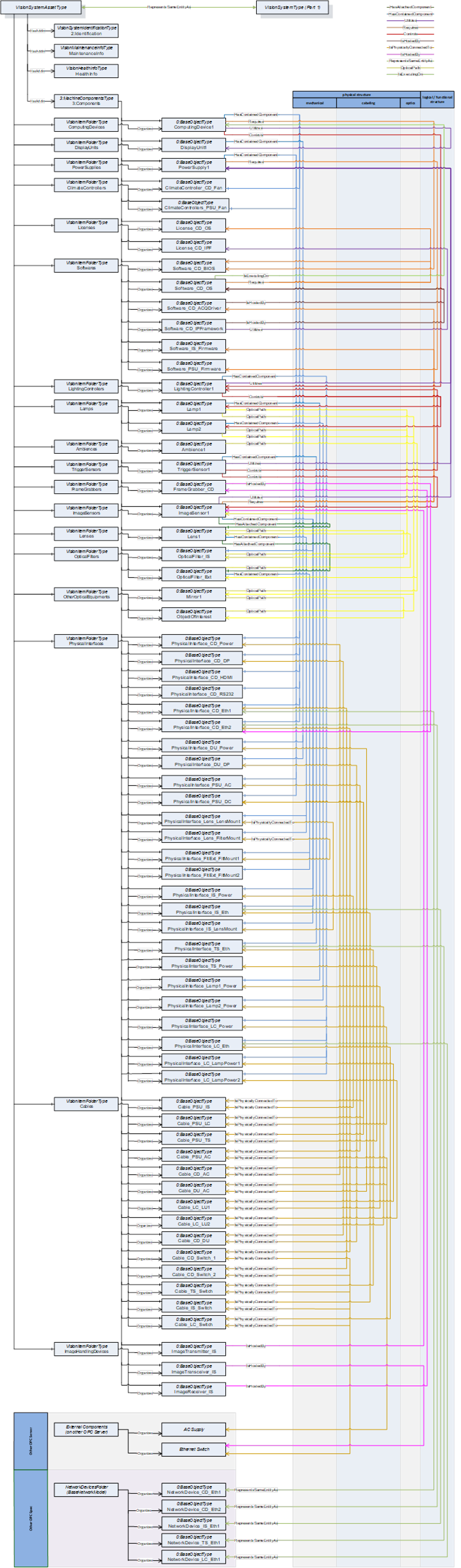
Finally using the modelling tools introduced in this companion specification along with the usage of OPC UA References as explained in the previous sections, the figure on the next page shows the entire address space model of the example used throughout this Annex.